• TOC

Background

Just a review of machine learning for myself (really busy recently, so …)

内容来自dive into deep learning, pattern recognition and machine learning, 网络。

Basics

Batch normalization

• Batch normalization: subtracting the batch mean and dividing by the batch standard deviation (2 trainable parameters for mean and standard deviation, mean->0, variance->1) to counter covariance shift (i.e. the distribution of input of training and testing are different) Batch Normalization: Accelerating Deep Network Training by Reducing Internal Covariate Shift 也方便optimization，而且各feature之间不会有莫名的侧重，注意是每个feature dimension分开进行batch normalization

• batch normalization 经常被每一层分别使用。batch size不能为1（因为这时输出总为0）。

• 这里说BN放在activation之后会更好一些

• batch normalization的优点是可以用更大的学习速率，减少了训练时间，初始化不那么重要，结果更好，是某种程度的regularization

• batch normalization在train和predict表现不一样，predict时是用的training时根据所有training set估计的population mean和variance，实现上是计算动态的值，during training keeps running estimates of its computed mean and variance

Layer normalization

• layer normalization和batch normalization类似，不过不是batch 那一维度（d=0）normalize，而是最后一个维度normalize, 作用是prevents the range of values in the layers from changing too much, which allows faster training and better generalization ability。

• batch normalization用在rnn上的话，得考虑不同sequence长度不同，而layer norm没有这个问题(one set of weight and bias shared over all time-steps)

• layer norm就是每个sample自己进行across feature 的layer层面的normalization，有自己的mean, variance。所以可以batch size为1, batch norm则是across minibatch 单个neuron来算

• MXNet’s ndarray比numpy的要多2特点，1是有automatic differentiation，2是支持在GPU, and distributed cloud architectures上的asynchronous computation.

• broadcast就是复制来填充新的维度

• missing data比如NaN可以用imputation(填充一些数)或者deletion来处理

• 使用x+=y或者z[:]=x可以在老地方设置新ndarray，节约内存

• scalar, vector, matrix, tensor: 0-, 1-, 2-, n-dimension

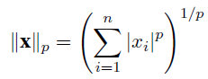
• $L_{p}$ norm:

• $L_{p}$norm的性质, for vectors in $C^{n}$ where $ 0 < r < p $：

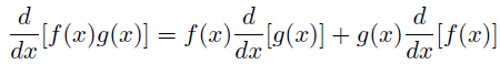
• calculus微积分: integration, differentiation

• product rule:

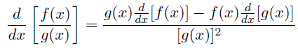
• quotient rule: 上面的是领导啊

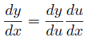
• chain rule:

• matrix calculus: 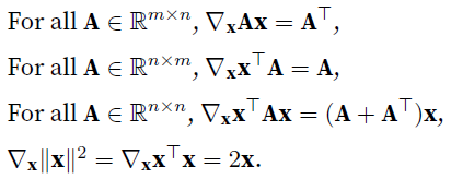matrix calculus wiki

• A gradient is a vector whose components are the partial derivatives of a multivariate function with respect to all its variables

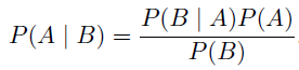
• Bayes’ Theorem:

• 推导

• dot product: a scalar; cross product: a vector

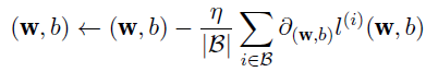
• stochastic gradient descent: update in direction of negative gradient of minibatch

• likelihood:

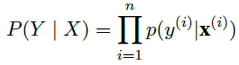
• 经常用negative log-likelihood来将maximize multiplication变成minimize sum

• minimizing squared error is equivalent to maximum likelihood estimation of a linear model under the assumption of additive Gaussian noise

• one-hot encoding: 1个1，其他补0

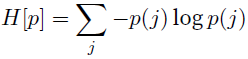
• entropy of a distribution p:

• cross-entropy is asymmetric: $H(p,q)=-\sum\limits_{x\in X}{p(x)\log q(x)}$

• minimize cross-entropy == maximize likelihood

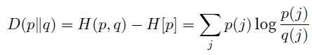
• Kullback-Leibler divergence (也叫relative entropy或者information gain) is the difference between cross-entropy and entropy:

• KL divergence is asymmetric and does not satisfy the triangle inequality

• Jensen-Shannon divergence: $}(P\parallel Q)={\frac {1}{2}}D(P\parallel M)+{\frac {1}{2}}D(Q\parallel M)$ where $M={\frac {1}{2}}(P+Q)$，这个JSD是symmetric的

• cross validation: split into k sets. do k experiments on (k-1 train, 1 validation), average the results

• forward propagation calculates and stores intermediate variables.

• 对于loss function $J$, 要计算偏导的$W$, $\frac{\partial J}{\partial W}=\frac{\partial J}{\partial O}*I^{T}+\lambda W$, 这里$O$是这个的output, $I$是这个的input，后面的term是regularization的导，这里也说明了为啥forward propagation要保留中间结果，此外注意activation function的导是elementwise multiplication，有些activation function对不同值的导得分别计算。training比prediction要占用更多内存

• Shift: distribution shift, covariate shift, label shift

• covariate shift correction: 后面说的只和feature $X$有关，和$y$是没有关系的。训练集来自$q(x)$，测试集来自$p(x)$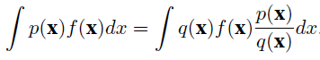，,所以训练时给$X$一个weight $\frac{p(x)}{q(x)}$即可。经常是来一个混合数据集，训练一个分类器来估计这个weight，logistics分类器好算。

• label shift correction:和上面一样，加个importance weights，说白了调整一下输出

• concept shift correction：经常是缓慢的，所以就把新的数据集，再训练更新一下模型即可。

• 确实的数据，可以用这个feature的mean填充

• Logarithms are useful for relative loss.除法变减法

• 对于复杂模型，有block这个概念表示特定的结构，可以是1层，几层或者整个模型。只要写好参数和forward函数即可。

• 模型有时候需要，也可以，使不同层之间绑定同样的参数，这时候backpropagation的gradient是被分享那一层各自的和，比如a->b->b->c，就是第一个b和第二个b的和

• chain rule (probability):

• cosine similarity，如果俩向量同向就是1

Hyperparameters

• 一般layer width (node个数)取2的幂，计算高效

Grid search

Random search

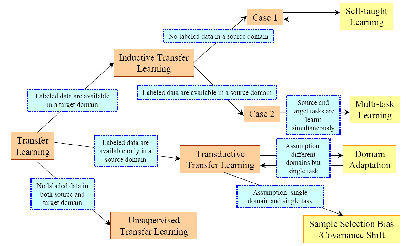
Transfer learning

• Chop off classification layers and replace with ones cater to ones’ needs. Freeze pretrained layers during training. Enable training on batch normalization layers as well may get better results.
• A Survey on Transfer Learning
• 

One-shot learning

Zero-shot learning

Curriculum learning

Objective function

Mean absolute error

Mean squared error

Cross-entropy loss

• $loss(x,class)=-\log(\frac{exp(x[class])}{\Sigma_{j}exp(x[j])})=-x[class]+\log(\Sigma_{j}exp(x[j]))$

Regularization

Weight decay

• 即L2 regularization
• encourages weight values to decay towards zero, unless supported by the data.
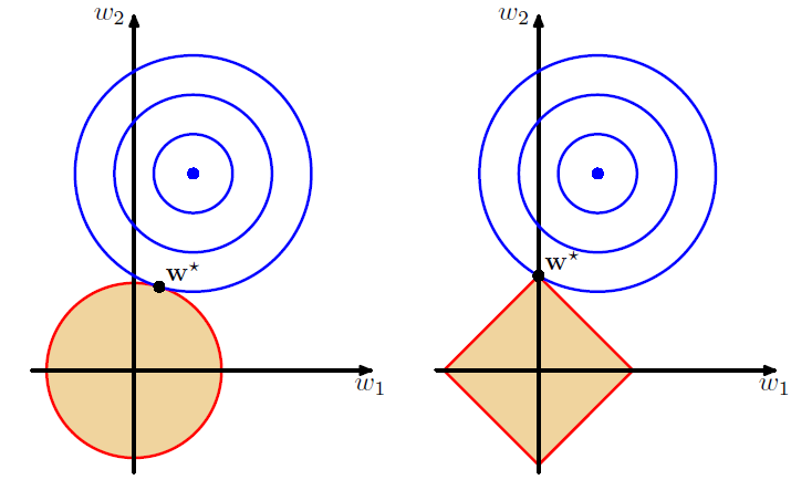
• 这是q=2,ridge，让weights distribute evenly, driven to small values
• q=1的话，lasso, if λ is sufficiently large, some of the coefficients $w_{j}$ are driven to zero, leading to a sparse model,比如右边lasso的 $w_{1}$

*

Dropout

• breaks up co-adaptation between layers
• in training, zeroing out each hidden unit with probability $p$, multiply by $\frac{1}{1-p}$ if kept, 这使得expected sum of weights, expected value of activation the same (这也是可以直接让p=0就用在test mode)
• in testing, no dropout
• 不同层可以不同dropout, a common trend is to set a lower dropout probability closer to the input layer

Label smoothing

• Use not hard target 1 and 0, but a smoothed distribution. Subtract $\epsilon$ from target class, and assign that to all the classes based on a distribution (i.e. sum to 1). So the new smoothed version is $q \prime (k \mid x)=(1-\epsilon)\delta_{k,y}+\epsilon u(k)$ (x is the sample, y is the target class, u is the class distribution) Rethinking the Inception Architecture for Computer Vision
• hurts perplexity, but improves accuracy and BLEU score.

Learning rate

Pick learning rate

• Let the learning rate increase linearly (multiply same number) from small to higher over each mini-batch, calculate the loss for each rate, plot it (log scale on learning rate), pick the learning rate that gives the greatest decline (the going-down slope for loss) Cyclical Learning Rates for Training Neural Networks

Warmup

• 对于区分度高的数据集，为了避免刚开始batches的data导致偏见，所以learning rate是线性从一个小的值增加到target 大小。https://stackoverflow.com/questions/55933867/what-does-learning-rate-warm-up-mean
• Accurate, Large Minibatch SGD: Training ImageNet in 1 Hour

Differential learning rate

• Use different learning rate for different layers of the model, e.g. use smaller learning rate for transfer learning pretrained-layers, use a larger learning rate for the new classification layer

Learning rate scheduling

• Start with a large learning rate, shrink after a number of iterations or after some conditions met (e.g. 3 epoch without improvement on loss)

Initialization

• 求偏导，简单例子，对于一个很多层dense的模型，偏导就是连乘，eigenvalues范围广，特别大或者特别小，这个是log-space不能解决的

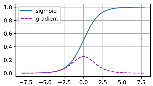
• Vanishing gradients: cause by比如用sigmoid做activation function,导数两头都趋于0，见图

• Exploding gradients：比如100个~Normal(0,1)的数连乘，output炸了，gradient也炸了，一发update，model参数就毁了

• Symmetry：全连接的话，同一层所有unit没差，所以如果初始化为同一个值就废了

• 普通可用的初始化，比如Uniform(-0.07, 0.07)或者Normal(mean=0, std=0.01)

Xavier initialization

• 为了满足variance经过一层后稳定，$\sigma^2$是某层$W$初始化后的的variance，对于forward propagation, 我们需要$n_{in}\sigma^2=1$，对于backward propagation，我们需要$n_{out}\sigma^2=1$，所以，选择满足
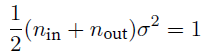
• 可以用mean是0，variance是$\sigma^2=\frac{2}{n_{in}+n_{out}}$的Gaussian distribution，也可以用uniform distribution $U(-\sqrt{\frac{6}{n_{in} + n_{out}}},\sqrt{\frac{6}{n_{in} + n_{out}}})$
• 注意到variance of uniform distribution $U(-a, a)$是$\int_{-a}^{a}(x-0)^2 \cdot f(x)dx=\int_{-a}^{a}x^2 \cdot \frac{1}{2a}dx=\frac{a^2}{3}$

Optimizer

• Gradient descent: go along the gradient, not applicable to extremely large model (memory, time)
• weight = weight - learning_rate * gradient​
• Stochastic gradient descent: pick a sample or a subset of data, go
• hessian matrix: a square matrix of second-order partial derivatives of a scalar-valued function, it describes the local curvature of a function of many variables.
• hessian matrix is symmetric, hessian matrix of a function f is the Jacobian matrix of the gradient of the function: H(f(x)) = J(∇f(x)).
• input k-dimensional vector and its output is a scalar:
• 1. eigenvalues of the functionʼs Hessian matrix at the zero-gradient position are all positive: local minimum
  2. eigenvalues of the functionʼs Hessian matrix at the zero-gradient position are all negative: local maximum
  3. eigenvalues of the functionʼs Hessian matrix at the zero-gradient position are negative and positive: saddle point
• convex functions are those where the eigenvalues of the Hessian are never negative
• Jensenʼs inequality: $f$函数是convex的，
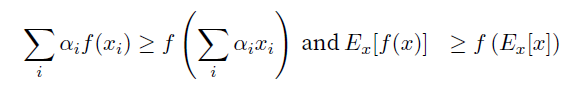
• convex函数没有local minima，不过可能有多个global minima或者没有global minima

Stochastic gradient descent

• 就是相对于gradient descent 用所有training set的平均梯度，这里用random一个sample的梯度
• stochastic gradient $∇f_{i}(\textbf{x})$ is the unbiased estimate of gradient $∇f(\textbf{x})$.

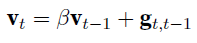
Momentum

• $\textbf{g}$ is gradient, $\textbf{v}$ is momentum, $\beta$ is between 0 and 1.

Adagrad

• 

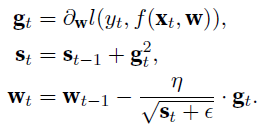
Adam

• 和SGD相比，对initial learning rate不敏感

Ensembles

• Combine multiple models’ predictions to produce a final result (can be a collection of different checkpoints of a single model or models of different structures)

Activations

ReLU

• $ReLU(z)=max(z,0)$
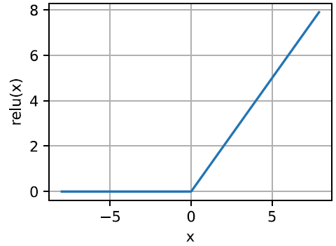
• mitigates vanishing gradient，不过还是有dying ReLU的问题

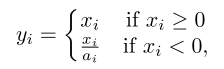
Leaky ReLU

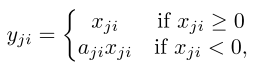
• 以下用$x_{ji}$ to denote the input of $i$th channel in $j$th example

• 就是negative部分也有一个小斜率

• $a_{i}$越大越接近ReLU，经验上可以取6~100

PReLU

• parametric rectified linear unit，和leaky一样， 不过$a_{i}$ is learned in the training via back propagation
• may suffer from severe overfitting issue in small scale dataset

RReLU

• Randomized Leaky Rectified Linear，就是把斜率从一个uniform $U(l,u)$里随机
• test phase取固定值，也就是$\frac{l+u}{2}$
• 在小数据集上表现不错，经常是training loss比别人大，但是test loss更小

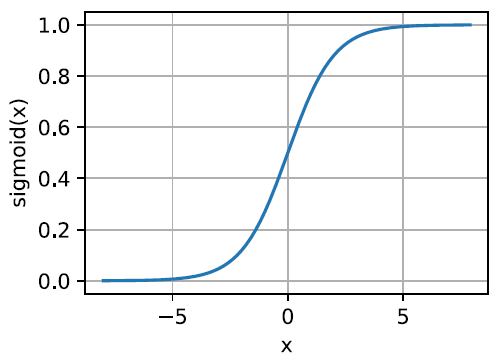
Sigmoid

• sigmoid是一类s型曲线，这一类都可能saturated
• 代表：logit function, logistic function(logit的inverse function)，hyperbolic tangent function
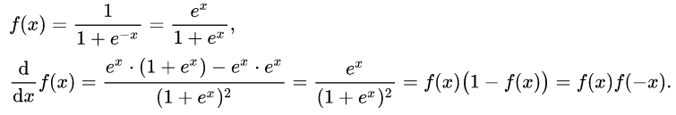
• logistic function值域 0 ~ 1 : $f(x)=\frac{1}{1+e^{-x}}$
• 求导$\frac{df}{dx}=f(x)(1-f(x))=f(x)f(-x)$过程
• 
• tanh (hyperbolic tangent) function: $f(x)=\frac{1-e^{-2x}}{1+e^{-2x}}$
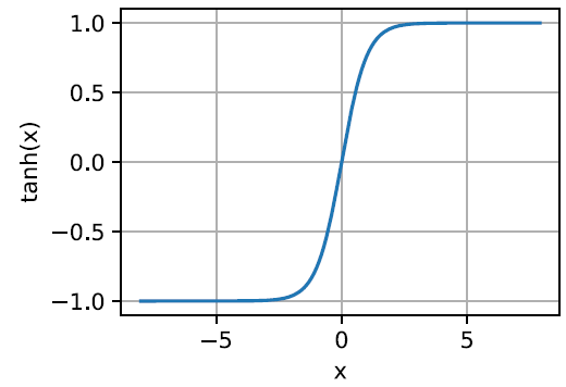
• tanh形状和logistic相似，不过tanh是原点对称的$\frac{df}{dx}=1-f^{2}(x)$

Softmax

• 计算

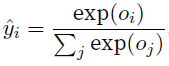
• softmax保证了each logit >=0且和为1

• 给softmax搭配cross entropy避免了exponential带来的数值overflow或者underflow问题

Convolutional neural network

• 更准确地说法是cross correlation: 各自对应位置乘积的和
• convolution就是先上下，左右flip，然后同上
• channel (filter, feature map, kernel):可以有好多个，输入rgb可以看成3channel.有些简单的kernel比如检测edge，[1, -1]就把横线都去了
• padding: 填充使得产出的结果形状的大小和输入相同，经常kernel是奇数的边长，就是为了padding时可以上下左右一致
• stride:减小resolution，以及体积
• 对于多个channel，3层input，就需要3层kernel，然后3层各自convolution后，加一起，成为一层，如果输出想多层，就多写个这种3层kernel，input,output的层数就发生了变化。总的来说，kernel是4维的，长宽进出
• 1*1 convolutional layer == fully connected layer
• pooling: 常见的有maximum, average
• pooling减轻了模型对location的敏感性，并且spatial downsampling，减少参数
• pooling没有参数，输入输出channel数是一样的
• 每一层convolutional layer后面都有activation function
• feature map: 就是一个filter应用于前一层后的output

Recurrent neural network

• May suffer vanishing or exploding gradient
• 可以用gradient clipping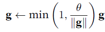gradient norm是在所有param上计算的
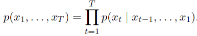
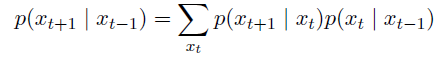
• Markov model: 一个first order markov model是
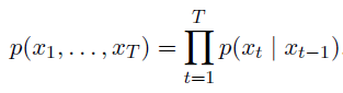
• if $x_{t}$只能取离散的值，那么有
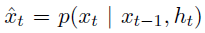
• autoregressive model:根据markov这样利用过去$\tau$个信息，计算下一位的条件概率
• latent autoregressive model:比如GRU, LSTM，更新一个latent state
• tokenization: word or character or bpe
• vocabulary 映射到0-n的数字，包括一些特殊的token, , ,
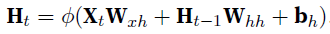
• RNN的参数并不随timestamp变化，
• error是softmax cross-entropy on each label
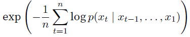
• perplexity:

GRU

• to deal with : 1. early observation is highly significant for predicting all future observations 2 , some symbols carry no pertinent observation (should skip) 3, logical break (reset internal states)
• reset gate $R_{t}$: capture short-term dependencies
• update gate $Z_{t}$: 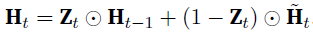capture long-term dependencies

LSTM

• Long short-term memory
• input gate
• forget gate
• output gate
• memory cell: entirely internal
• Can be bidirectional (just stack 2 lstm together, with input of opposite direction)

Encoder-decoder

• a neural network design pattern, encoder -> state(several vector i.e. tensors) -> decoder
• An encoder is a network (FC, CNN, RNN, etc.) that takes the input, and outputs a feature map, a vector or a tensor
• An decoder is a network (usually the same network structure as encoder) that takes the feature vector from the encoder, and gives the best closest match to the actual input or intended output.
• sequence-to-sequence model is based on encoder-decoder architecture, both encoder and decoder are RNNs
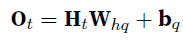
• 对于一个encoder-decoder模型，内部是这样的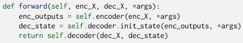hidden state of the encoder is used directly to initialize the decoder hidden state to pass information from the encoder to the decoder

Computer vision

Data augmentation

general

• Mixup: superimpose e.g. 2 images together with a weight respectively e.g. 0.3, 0.7, classification loss modified to mean of the 2 class (with true labels not as 1s, but as 0.3, 0.7) mixup: Beyond Empirical Risk Minimization

for image

• Change to RGB, HSV, YUV, LAB color spaces
• Change the brightness, contrast, saturation and hue: grayscale
• Affine transformation: horizontal or vertical flip, rotation, rescale, shear, translate
• Crop

for text

• Back-translation for machine translation task, use a translator from opposite direction and generate (synthetic source data, monolingual target data) dataset

for audio

• SoX effects
• Change to spectrograms, then apply time warping, frequency masking (randomly remove a set of frequencies), time masking SpecAugment: A Simple Data Augmentation Method for Automatic Speech Recognition

Pooling

• Natural language processing

• beam search: $ \mid Y \mid $这么多的词汇，很简单，就是每一层都挑前一层$k * \mid Y \mid $中挑最可能的k个。最后，收获的不是k个，而是$k * L$个，L是最长搜索的长度，e.g. a, a->b, a->b->c, 最后这些还用perplexity在candidates中来挑选一下最可能的。

• one-hot 不能很好的体现word之间的相似性，任意2个vector的cosine都是0

Embeddings

• The technique of mapping words to vectors of real numbers is known as word embedding.
• word embedding可以给下游任务用，也可以直接用来找近义词或者类比（biggest = big + worst - bad）
• one-hot的维度是词汇量大小，sparse and high-dimensional，训练的embedding几维其实就是几个column，n个词汇，d维表示出来就是$n*d$的2维矩阵，所以很dense，一般就几百维

Word2vec

• Word2vec is a group of related models that are used to produce word embeddings. These models are shallow, two-layer neural networks that are trained to reconstruct linguistic contexts of words. Word2vec takes as its input a large corpus of text and produces a vector space, typically of several hundred dimensions, with each unique word in the corpus being assigned a corresponding vector in the space. Word vectors are positioned in the vector space such that words that share common contexts in the corpus are located close to one another in the space.
• 训练时，会抑制那些出现频率高的词，比如the，所以出现频率越高，训练时某句中被dropout的概率越大

Skip-gram model

• central target word中间的word，而context word是central target word两侧window size以内的词
• 每个词有两个d维向量，一个$\textbf v_{i}$给central target word，一个$\textbf u_{i}$给context word
• 下标是在字典里的index，${0,1,…,\mid V\mid-1}$，其中$V$是vocabulary
• skip-gram不考虑复杂的，也无关距离，就是是不是context的一元条件概率，$w_{o}$是context word, $w_{c}$是target word。
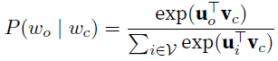
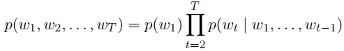
• $T$ is the length of text sequence, $m$ is window size, the joint probability of generating all context words given the central target word is
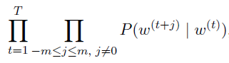
• 训练时候就是minimize上面这个probability的-log，然后对$\textbf u_{i}$, $\textbf v_{i}$各自求偏导来update

CBOW model

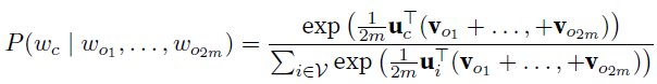
• skip-gram是给central target word下产生context word的概率，CBOW反过来，给context word，生成中间的target word
• 以下$\textbf u_{i}$是target word, $\textbf v_{i}$是context word，和skip-gram相反。windows size $m$,方式其实和skip-gram类似，不过因为context word很多，所以求平均向量来相乘
• 同样的，对于长度$T$的sequence，likelihood function如下
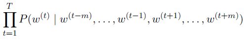
• 同样的，minimize -log
• 推荐的windows size是10 for skip-gram and 5 for CBOW
• 一般来说，central target word vector in the skip-gram model is generally used as the representation vector of a word，而CBOW用的是context word vector

Negative sampling

• 注意到上面skip-gram和CBOW我们每次softmax都要计算字典大小$\mid V \mid $这么多。所以用两种approximation的方法，negative sampling和hierarchical softmax
• 本质上这里就是换了一个loss function。多分类退化成了近似的二分类问题。
• 解释论文，这个文章给了一种需要target word和context word不同vector的理由，因为自己和自己相近出现是很困难的，但是$v \cdot v$很小不符合逻辑。
• 不用conditional probability而用joint probability了，$D=1$指文本中有这个上下文，如果没有就是$D=0$，也就是negative samples
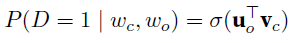
• 这里$\sigma$函数是sigmoid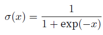个人认为主要好处是-log可以化简
• 老样子，对于长度$T$的文本，joint probability
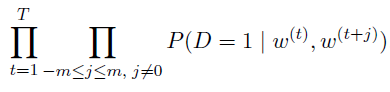
• 如果只是maximize这个，就都是相同的1了，所以需要negative samples
• 最后变成了如下，随机K个negative samples
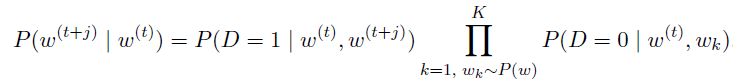
• 现在gradient计算跟$\mid V \mid $没关系了，和K线性相关

Hierarchical softmax

• 每个叶子节点是个word，$L(w)$是w的深度，$n(w,j)$是这个路径上$j^{th}$节点
• 改写成
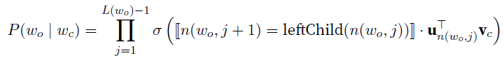
• 其中条件为真，$[![x]!]=1$，否则为$-1$
• 现在是$\log_{2}{\mid V \mid }$

GloVe

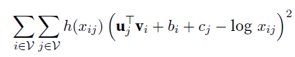
• use square loss，数以$w_{i}$为central target word的那些context word的个数，比如某个word $w_{j}$，那么这个个数记为$x_{ij}$，注意到两个词互为context，所以$x_{ij}=x_{ji}$，这带来一个好处，2 vectors相等（实际中训练后俩vector因为初始化不一样，所以训练后不一样，取sum作为最后训练好的的embedding）
• 令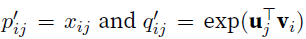，$p’$是我们的目标，$q’$是要训练的那俩vector，此外还有俩bias标量参数，一个给target word $b_{i}$, 一个给context word $c_{i}$. The weight function $h(x)$ is a monotone increasing function with the range [0; 1].
• loss function is

Subword embedding

• 欧洲很多语言词性变化很多（morphology词态学），但是意思相近，简单的每个词对应某向量就浪费了这种信息。用subword embedding可以生成训练中没见过的词

fastText

• 给每个单词加上<>，然后按照character取长度3-6的那些subword，然后自己本身<myself>也是一个subword，这些subword都按照skip-gram训练词向量，最后central word vector $\textbf u_{w}$就是其所有subword的向量和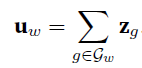
• 缺点是vocabulary变大很多

BPE

• Byte pair encoding: the most common pair of consecutive bytes of data is replaced with a byte that does not occur within that data, do this recursively Neural Machine Translation of Rare Words with Subword Units
• 从length=1的symbol是开始，也就是字母，greedy

BERT (Bidirectional Encoder Representations from Transformers)

• 本质上word embedding是种粗浅的pretrain，而且word2vec, GloVe是context无关的，因为单词一词多义，所以context-sensitive的语言模型很有价值
• 在context-sensitive的语言模型中，ELMo是task-specific, GPT更好的一点就是它是task-agnostic(不可知的)，不过GPT只是一侧context，从左到右，左边一样的话对应的vector就一样，不如ELMo，BERT天然双向context。在ELMo中，加的pretrained model被froze，不过GPT中所有参数都会被fine-tune.
• classification token <cls>，separation token <sep>
• The embeddings of the BERT input sequence are the sum of the token embeddings, segment embeddings, and positional embeddings这仨都是要训练的
• pretraining包含两个tasks，masked language modeling 和next sentence prediction
• masked language modeling就是mask某些词为<mask>，然后来预测这个token。loss可以是cross-entropy
• next sentence prediction则是判断两个句子是否是连着的，binary classification，也可用cross-entropy loss
• BERT可以被用于大量不同任务，加上fully-connected layer，这是要train的，而本身的pretrained parameters也要fine-tune。Parameters that are only related to pretraining loss will not be updated during finetuning，指的是按照masked language modelling loss和next sentence prediction loss训练的俩MLPs
• 一般是BERT representation of <cls>这个token被用来transform，比如扔到一个mlp中去输出个分数或类别
• 一般来说BERT不适合text generation，因为虽然可以全都<mask>，然后随便生成。但是不如GPT-2那种从左到右生成。

ELMo (Embeddings from Language Models)

• each token is assigned a representation that is a function of the entire input sentence.

GPT

• N-grams

• 语言模型language model:

• Laplace smoothing (additive smoothing): 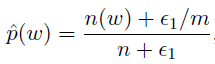,这里m是categories数量，所以估计值会在原本的概率和1/m的均匀分布之间，$\alpha$经常取0~1之间的数，如果是1的话，这个也叫做add-one smoothing

• Metrics

BLEU

TER

Attention

• Attention Is All You Need

• Attention is a generalized pooling method with bias alignment over inputs.

• 参数少，速度快（可并行），效果好

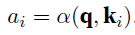
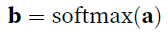
• attention layer有个key-value pairs $\bf (k_{1}, v_{1})..(k_{n}, v_{n})$组成的memory，输入query $\bf{q}$，然后用score function $\alpha$计算query和key的相似度，然后输出对应的value作为output $\bf o$

• 

• 两种常见attention layer,都可以内含有dropout: dot product attention (multiplicative) and multilayer perceptron (additive) attention.前者score function就是点乘（要求query和keys的维度一样），后者则有个可训练的hidden layer的MLP，输出一个数

• dimension of the keys $d_{k}$, multiplicative attention is much faster and more space-efficient in practice, since it can be implemented using highly optimized matrix multiplication code. Additive attention outperforms dot product attention without scaling for larger values of $d_{k}$ (所以原论文里用scaled dot product attention，给点乘后的结果乘了一个$\frac{1}{\sqrt{d_{k}}}$的参数)

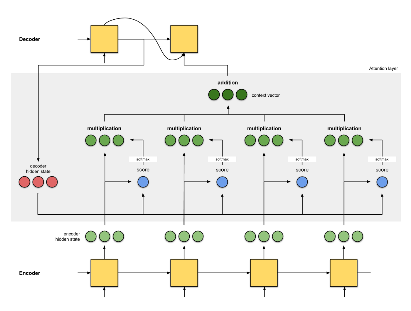
• seq2seq with attention mechanism: encoder没变化。during the decoding, the decoder output from the previous timestep $t-1$ is used as the query. The output of the attention model is viewed as the context information, and such context is concatenated with the decoder input Dt. Finally, we feed the concatenation into the decoder.下图没有 concat，但是基本差不多

  

• The decoder of the seq2seq with attention model passes three items from the encoder:

• 1. the encoder outputs of all timesteps: they are used as the attention layerʼs memory with identical keys and values;
  2. the hidden state of the encoderʼs final timestep: it is used as the initial decoderʼs hidden state;
  3. the encoder valid length: so the attention layer will not consider the padding tokens with in the encoder outputs.

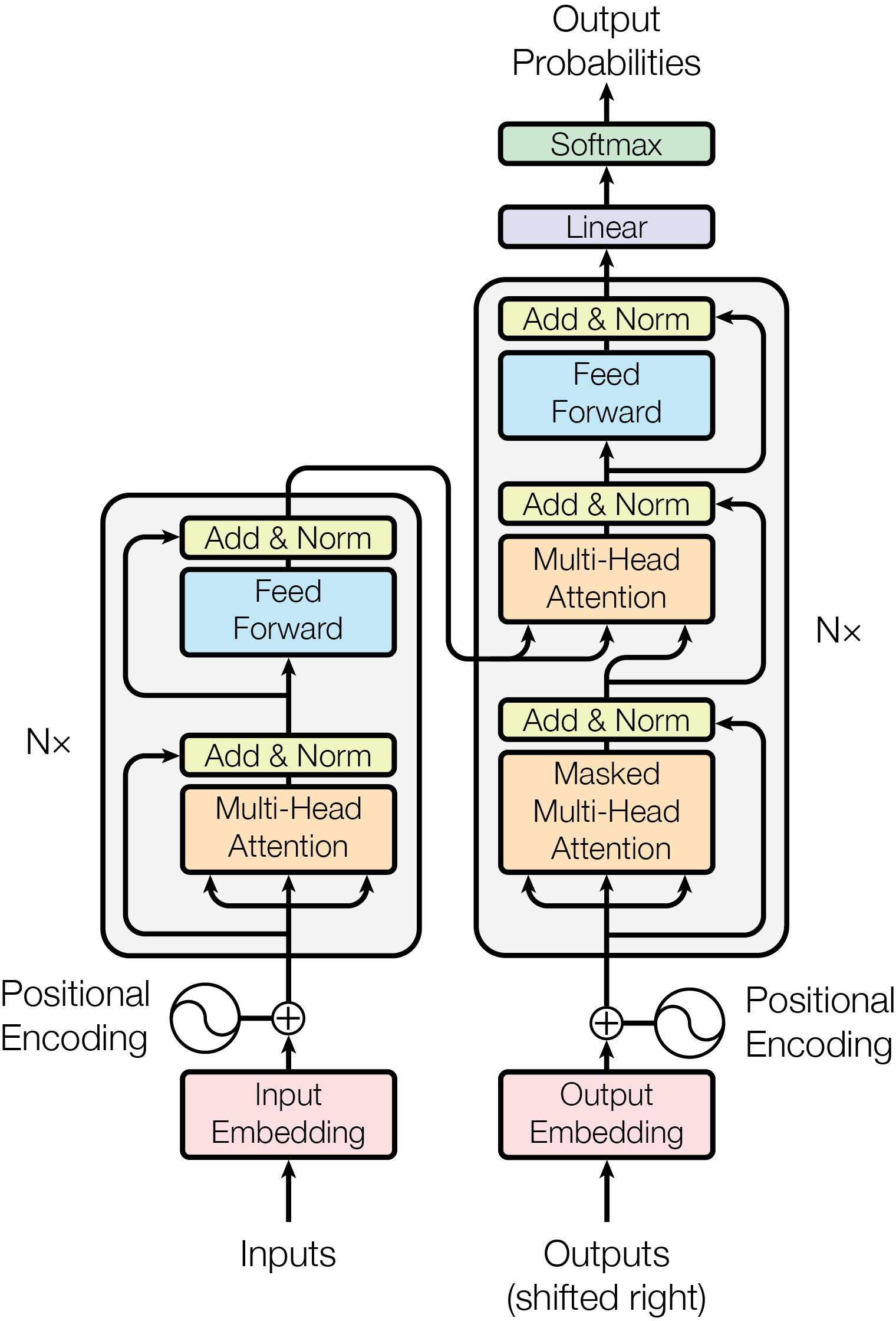
• transformer:主要是加了3个东西，

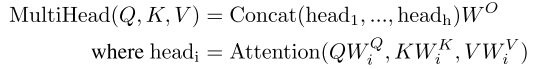
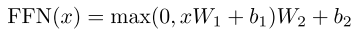
• 1. transformer block:包含两种sublayers，multi-head attention layer and position-wise feed-forward network layers
  2. add and norm: a residual structure and a layer normalization，注意到右边式子括号中是residual，外面是layer norm
  3. position encoding: 唯一add positional information的地方

• 

• self-attention model is a normal attention model, with its query, its key, and its value being copied exactly the same from each item of the sequential inputs. output items of a self-attention layer can be computed in parallel. Self attention is a mechanism relating different positions of a single sequence in order to compute a representation of the sequence.

• multi-head attention: contain parallel self-attention layers (head), 可以是any attention (e.g. dot product attention, mlp attention)

• 在transformer中multi-head attention用在了3处，1是encoder-decoder attention, queries come from the previous decoder layer, and the memory keys and values come from the output of the encoder。2是self-attention in encoder，all of the keys, values and queries come from output of the previous layer in the encoder。3是self-attention in decoder, 类似

• position-wise feed-forward networks:3-d inputs with shape (batch size, sequence length, feature size), consists of two dense layers, equivalent to applying two $1*1$ convolution layers

• 这个feed-forward networks applied to each position separately and identically,不过当然不同层的参数不一样。本质式子就是俩线性变换夹了一个ReLU，

• add and norm: X as the original input in the residual network, and Y as the outputs from either the multi-head attention layer or the position-wise FFN network. In addition, we apply dropout on Y for regularization.

• position encoding: 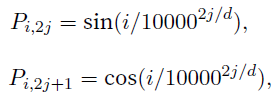$i$ refers to the order in the sentence, and $j$ refers to the position along the embedding vector dimension, $d$是dimension of embedding。这个函数应该更容易把握relative positions，并且没有sequence长度限制，不过也可以用别的，比如learned ones ，一些解释https://www.zhihu.com/question/347678607

• https://medium.com/@pkqiang49/%E4%B8%80%E6%96%87%E7%9C%8B%E6%87%82-attention-%E6%9C%AC%E8%B4%A8%E5%8E%9F%E7%90%86-3%E5%A4%A7%E4%BC%98%E7%82%B9-5%E5%A4%A7%E7%B1%BB%E5%9E%8B-e4fbe4b6d030
• A Decomposable Attention Model for Natural Language Inference这里提出一种结构，可以parameter少，还并行性好，结果还很好，3 steps: attending, comparing, aggregating.

self-attention

• https://towardsdatascience.com/illustrated-self-attention-2d627e33b20a
• 

target-attention

multi-head attention

Unsupervised machine translation

• https://github.com/facebookresearch/MUSE

• Word Translation Without Parallel Data

• Unsupervised Machine Translation Using Monolingual Corpora Only

• starts with an unsupervised naïve translation model obtained by making word-by-word translation of sentences using a parallel dictionary learned in an unsupervised way

• train the encoder and decoder by reconstructing a sentence in a particular domain, given a noisy version （避免直接copy）of the same sentence in the same or in the other domain （重建或翻译）其中result of a translation with the model at the previous iteration in the case of the translation task.

• 此外还训练一个神经网络discriminator，encoder需要fool这个网络(让它判断不了输入语言ADVERSARIAL TRAINING)

GAN

• generative adversarial nets - paper
• 本质是个minmax，$D$是discriminator, $G$ is generator.
• $y$ is label, true 1 fake 0, $\textbf{x}$ is inputs, $D$ minimize
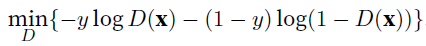
• $\textbf{z}$ is latent variable, 经常是random来生成data
• $G$ maximize 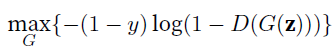但是实现的时候，我们实际上是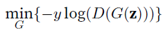， 特点是D的loss提供了training signal给G(当然，因为一个max，一个想min，所以把label由1变0)
• vanilla GAN couldn’t model all modes on a simple 2D dataset VEEGAN: Reducing Mode Collapse in GANs using Implicit Variational Learning

Reinforcement learning

Basics

• course: https://github.com/huggingface/deep-rl-class

• loop: state0, action0, reward1, state1, action1, reward2 …

• state: complete description of the world, no hidden information

• observation: partial description of the state of the world

• goal: maximize expected cumulative reward

• policy: tells what action to take given a state

• task:

  • episodic

  • continuing

• method:

  • policy-based (learn which action to take given a state)

    • deterministic 给定 state s 会选择固定某个 action a

    • stochatistic:  output a probability distribution over actions

  • value-based (maps a state to the expected value of being at that state)

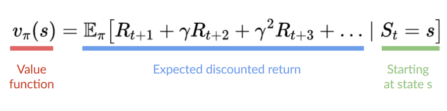    • 随时间 reward 有一个衰减， γ < 1
    • 这时 policy 是个简单的人为确定的策略

• value-based methods

  • Monte Carlo: update the value function from a complete episode, and so we use the actual accurate discounted return of this episode (获得实际的一个 episode 的 reward)

  • Temporal Difference: update the value function from a step, so we replace Gt that we don’t have with an estimated return called TD target （获得一个 action的 reward 以及对于下个 state 的估计来更新现在 state，基于 bellman equation）

• Bellman equation:

  • 

Q-learning

• Trains Q-Function (an action-value function) which internally is a Q-table that contains all the state-action pair values

• 一般 q-table 都初始化成 0

Recommender system

Basics

• 召回即触发 (recall and trigger)
• multi-hot: 介于 label encoding 和 one-hot 之间 https://stats.stackexchange.com/questions/467633/what-exactly-is-multi-hot-encoding-and-how-is-it-different-from-one-hot

CF (collaborative filtering)

• 头部效应明显，处理稀疏向量能力弱，泛化差

UserCF

• Drawbacks: user num is much larger than item num, and storage of a similarity matix is expensive, grow by O(n^2), sparse, especially for new users low rate

ItemCF

• 一个用户 * 物品的m*n矩阵，物品相似度，根据正反馈物品推荐topk
• 相较而言，UserCF适合发现新热点，ItemCF适合稳定的兴趣点

Matrix factorization

• MF is 1-st order of FM (factorization machine)

• 用更稠密的隐向量，利用了全局信息，一定程度上比CF更好的处理稀疏问题

• 说白了就是把m*n matrix factorized into m*k and k*n,k is the size of the hidden vector, the size is chosen by trade off generalization, calculation and expression capability

• When recommendation, just dot multiply the user vector with item vector

• 2 methods: SVD and gradient descent

• SVD needs co-occurrence matrix to be dense, however, it is very unlikely in the real case, so fill-in; Compution complexity O(m*n^2)

• Gradient descent objective function, where K is the set of user ratings

• \[min_{q^{*},p^{*}}\Sigma_{(u,i) \in K}{(r_{ui} - q_{i}^{T}p_{u})}^{2}\]

• to counter over-fitting, we can add regularization

• \[\lambda(\lVert q_{i} \rVert^{2} + \lVert p_{u} \rVert^{2})\]

• MF的空间复杂度降低为(n+m)*k

• drawbacks: 不方便加入用户，物品和context信息，同时在缺乏用户历史行为时也表现不佳

逻辑回归

• logistics regressio assumes dependent variable y obeys Bernoulli distribution偏心硬币, linear regression assumes y obeys gaussian distribution, 所以logistics regression更符合预测CTR (click through rate)要求

• 辛普森悖论，就是多一个维度时，都表现更好的a，在汇总数据后反而表现差，本质是维度不是均匀的。所以不能轻易合并高维数据，会损失信息

• 本质就是特征给个权重，相乘以后用非线性函数打个分，所以不具有特征交叉生成高维组合特征的能力

• POLY2：一种特征两两交叉的方法，给特征组合一个权重，不过只是治标，而且训练复杂度提升，大量交叉特征很稀疏，根本没有足够训练数据

• \[\Phi POLY2(w,x)=\Sigma_{j_{1}=1}^{n-1}{\Sigma_{j_{2}=j_{1}+1}^{n}{w_{n(j_{1}, j_{2})}x_{j_{1}}x_{j_{2}}}}\]

Factorization machine

• 以下是FM的2阶版本

• \[\Phi FM(w,x)=\Sigma_{j_{1}=1}^{n-1}{\Sigma_{j_{2}=j_{1}+1}^{n}{(w_{j_{1}}\cdot w_{j_{2}})x_{j_{1}}x_{j_{2}}}}\]

• 每个特征学习一个latent vector, 隐向量的内积作为交叉特征的权重，权重参数数量从n^2 -> kn

• FFM, 引入了field-aware特征域感知，表达能力更强

• \[\Phi FFM(w,x)=\Sigma_{j_{1}=1}^{n-1}{\Sigma_{j_{2}=j_{1}+1}^{n}{(w_{j_{1},f_{2}}\cdot w_{j_{2},f_{1}})x_{j_{1}}x_{j_{2}}}}\]

• 说白了就是特征变成一组，看菜吃饭

• 参数变成n*f*k，其中f是特征域个数，训练复杂度kn^2

• FM and FFM可以拓展到高维，不过组合爆炸，现实少用

GBDT + LR

• GBDT就是构建新的离散特征向量的方法，LR就是logistics regression，和前者是分开的，不用梯度回传啥的
• GBDT就是gradient boosting decision tree，

AutoRec

• AutoEncoder + CF的single hidden layer 的神经网络

• autoencoder 的objective function如下

• \[\min_{\theta}\Sigma_{r\in S}{\lVert}r-h(r;\theta)\rVert_{2}^{2}\]

• 重建函数 h 的参数量一般远小于输入向量的维度

• 经典的模型是3层，input, hidden and output

• \[h(r;\theta)=f(W\cdot g(Vr + \mu)+b)\]

• 其中f，g都是激活函数，而V，输入层到隐层的参数，W是隐层到输出层的参数矩阵

• 可以加上L2 norm，就用普通的提督反向传播就可以训练

Deep Crossing

• 4 种 layers
• embedding layer： embedding一般是不会啊one-hot or multi-hot的稀疏响亮转换成稠密的向量，数值型feature可以不用embedding
• stacking layer： 把embeddign 和数值型特征连接到一起
• multiple residual units layer: 这个Res结构实现了feature的交叉重组，可以很深，所以就是deep crossing
• scoring layer: normally logistics for CTR predict or softmax for image classification

NeuralCF

• https://paperswithcode.com/paper/neural-collaborative-filtering
• 利用神经网络来替代协同过滤的内积来进行特征交叉

PNN

• 相对于 deep crossing 模型，就是把 stacking layer 换成 product layer，说白了就是更好的交叉特征
• IPNN，就是 inner product
• OPNN, 就是 outer product，其中外积操作会让模型复杂度从 M （向量的维度）变成 $M^{2}$,可以通过 superposition 来解决，这个操作相当于一个 average pooling，然后再进行外积互操作
• average pooling一般用在同类的 embedding 中，否则会模糊很重要的信息

Wide & Deep

• Wide 主要是记忆，而 deep 则更好的泛化
• 单输入层的 Wide部分：已安装应用和曝光应用 2 个
• Deep 部分：全量特征
• 
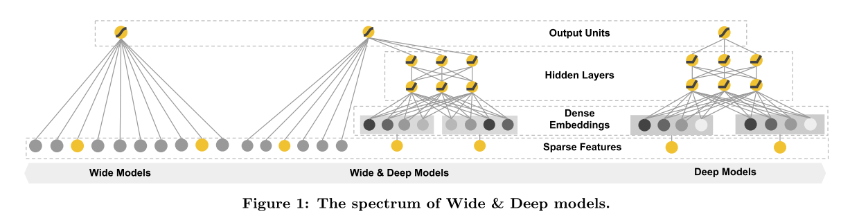
• Deep & cross：本质就是cross layer进行特征交叉，替代掉 wide 部分

FNN, DeepFM, NFM

FNN

• 本质在于 embedding 的改进，普通 embedding 训练非常慢
• embedding 训练收敛慢：
  1. 参数数量大
  2. 稀疏，只有非0特征连着的embedding会更新
• 使用 FM 模型训练好特征的隐向量来初始化 embedding 层，然后训练 embedding

DeepFM

• FM 替换 wide
• FM 和 deep 共享相同的 embedding 层

AFM, DIN

AFM

• 注意力机制替代 sum pooling
• 给两两交叉特征层加一个 attention 然后输出 $f_{Att}{j(f_{PI}{(\epsilon)})=\Sigma_{(i,j)\in R_{x}}{a_{ij}(v_{i}\odot v_{j})x_{i}x_{j}}}$
• 注意力网络是单个全连接层加 softmax，要学习的就是 W, b, h
• $a\prime_{ij}=h^{T}ReLU(W(v_{i}\odot v_{j})x_{i}x_{j}+b)$
• $a_{ij}=\frac{\exp(a\prime_{ij})}{\Sigma_{(i,j)\in R_{x}}{\exp (a\prime_{ij})}}$
• 注意力网络跟大家一块训练即可

DIN

• item特征组老样子，user特征组由 sum 变成 weighted sum，加上了 attention 的权重，本质就是加了个 attention unit
• attention unit：输入 2 embedding，计算 element-wise 减，这三者连接在一起，输入全连接层，然后单神经元输出一个 score
• attention 结构并不复杂，但是有效，应该是因为什么和什么相关的业务信息被attention表示了，比如item id和用户浏览过的item id发生作用，而不需要所有embedding都发生关系，那样训练困难，耗的资源多，逻辑上也不显然

DIEN

• 本质是相对于 DIN 加了时间的序列
• 额外加了一个兴趣进化网络，分为三层，从低到高
  1. behaviour layer
  2. interest extraction layer
  3. interest evolving layer
• interest extraction layer: 用的 GRU，这个没有RNN梯度消失的问题，也没有LSTM那么多参数，收敛速度更快
• interest evolving layer：主要是加上了 attention

DRN

• 强化学习模型，好处是online
• Deep Q-Network，quality，给行动打分
• 
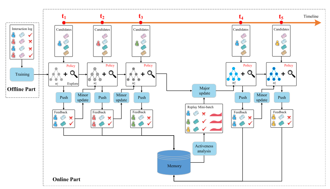
• 离线用历史数据训练一个初始化模型
• t1 -> t2 推送服务
• t2 微更新 （DBGDA）
• t4 主更新，就是重新训练
• t5 重复
• dueling bandit gradient descent algorithm:
  1. 对于网络 Q 的参数$W$，增加一个随机的扰动，得到新的模型参数$\tilde{W}$，这个叫探索网络
  2. 新老网络分别生成推荐结果$L$ $\tilde{L}$，然后俩进行 interleaving后推给用户
  3. 好则用，不好则留，迭代

Embeddings

• 主要用在3个方面
  1. 网络中的 embedding 层，（和网络整体训练虽好，但是很多时候收敛太慢了，所以经常是 embedding 单独进行预训练）
  2. embedding 和别的特征向量进行拼接
  3. 通过 embedding 相似度直接进行召回 （这个要求的是 user, item的向量处于同一个向量空间，这样就可以直接搜索最近邻，不用进行点积运算，用locality sensitie hashing）

Item2vec

• 和 word2vec 差不多，不过去掉了时间窗口（或者说markov），用用户历史记录序列中所有的item，两两有关
• 对于一个长度为K的用户历史记录 $w_{1},…,w_{K}$，objective function: $\frac{1}{K}\Sigma_{i=1}^{K}{\Sigma_{j\neq i}^{K}{\log p(w_{j}\lvert w_{i})}}$
• 主要是用于序列型数据

Graph embedding

• 可以处理网络型数据
• 包含结构信息和局部相似性信息

DeepWalk

• 构建方法：
  1. 用户行为序列构建有向图，多次连续出现的物品对，那么对应的边的权重被加强
  2. 随机起始点，随机游走，产生物品序列，概率就是按照出边的权的比例来
  3. 新的物品序列输入 word2vec，产生 embedding

Node2vec

• 网络具有：
  1. 同质性 homophily，相近节点 embedding 相似，游走更偏 DFS，商品（同品类，同属性）
  2. 结构性 structural equivalence，结构相似的节点 embedding 相似，游走更偏 BFS，商品（都是爆款，都是凑单）
• 调整超参数控制游走，可以产生不同侧重的 embedding，然后都用来后续训练

locality sensitive hashing 局部敏感哈希

• 本质是高维空间的点到低维空间的映射，满足高维相近低维也一定相近，但是远的也有一定的概率变成相近的
• 对于一个 k 维函数，让它计算一下和 k*m 矩阵的运算，就得到一个 m 维的向量，这个 矩阵其实就是 m 个hash 函数，对于生成的向量v，在它 m 个层面进行分桶（$[\frac{v}{w}]$，就是除以桶的宽度然后取整），这样我们就知道了相近的点就是在各个维度相近的桶里，这样查找就会非常快
• 使用几个hash函数，这些hash函数是用 and, or都是工程上面的权衡

Explore and exploit

• 推荐不能太过分，也要注意用户新兴趣的培养，多样性，同时对物品冷启也有好处
• 分3类：
  1. 传统的：$\epsilon-Greedy$, Thompson Sampling (适用于偏心硬币，CTR) and UCB (upper confidence bound)
  2. 个性化的：LinUCB
  3. 模型的：DRN

工程实现

大数据

• 1. 批处理：HDFS + map reduce，延迟较大
  2. 流计算：Storm, Flink，延迟小，灵活性大
  3. lambda：批处理（离线处理） + 流计算（实时流），落盘前会进行合并和纠错校验
  4. kappa：把批处理看作是时间窗口比较大的流处理，存储原始数据+数据重播

模型训练 （分布式）

• 1. Spark MLlib:全局广播，同步阻断式，慢，确保一致性
  2. Parameter server:异步非阻断式，速度快，一致性有损（某个），多server，一致性hash，参数范围拉取和推送

离线评估

• 我们需要的是所有 item 的一种排序，所以直接序列的评估相对于 ctr 之类的可能更好一点

P-R 曲线

• precision - recall curve，通过变化阈值生成（正负样本的阈值）
• AUC - area under curve 来比较曲线的优劣，而不是单个点

ROC curve

• receiver operating characteristic curve
• 横坐标 false positive rate， 纵坐标 true positive rate
• 也是通过变化正负样本与之来画的
• 也用 auc

Normalized Discounted Cumulative Gain (NDCG)

• 相比较于 precision, recall，更多地考虑了排序顺序；目标 item 越靠前，分数越高
• $rel_i$ 是 item i 的 relevance (得分), $p$ 是在 rank position $p$ , IDCG 是最理想情况，最大值 1.0

\[DCG_{p}=\sum_{i=1}^{p}{\frac{rel_i}{\log_{2}(i + 1)}}\]

$$

\[IDCG_{p}=\sum_{i=1}^{|REL_{p}|}{\frac{2^{rel_i}-1}{\log_{2}{(i+1)}}}\]

$$

\[nDCG_{p}=\frac{DCG_{p}}{IDCG_{p}}\]

mAP

• mean average precision

• 对于每个用户，对样本进行排序，然后对于所有正样本处的 precision进行平均，得到一个值 ap，对所有用户进行平均，得到mAP

• roc 和 p-r 都是直接对样本排序，只有mAP 需要分用户对样本排序

  replay

• 注意防止穿越

• 尽量让离线评估贴近线上结果，模型需要化静态为动态

• replay 就是接收到样本就更新的精准线上仿真

线上评估

• 用户层面不同层正交，同层互斥

• interleaving: 在 attest 之前迅速的减小需要检验的算法集，不区分用户群体，所以不会有群体差异。同时提供算法a和b的结果，不过交叉在一起（用户不知道），当然算法结果前后位置顺序得保证公平出现

• interleaving 具有比 attest 更高的灵敏度，也更容易出现置信的数据，其结果和 abtest 也很有相关性

• interleaving 缺点是实现有挑战，而且实验结果不是实际的那些（时长，留存）

• 总的一个关系是 离线 -> replay -> interleaving -> abtest 真实性和消耗资源逐渐变高

Appendix

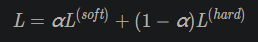
• 知识蒸馏：模型压缩，用小模型模拟 a pre-trained, larger model (or ensemble of models)，引入一个变量softmax temperature $T$，$T$经常是1~20，$p_i = \frac{exp\left(\frac{z_i}{T}\right)}{\sum_{j} \exp\left(\frac{z_j}{T}\right)}$。两个新的超参数$\alpha, \beta$，其中$\beta$一般是$1-\alpha$，soft target包含的信息量更大。

• 步骤：1、训练大模型：先用hard target，也就是正常的label训练大模型。 2、计算soft target：利用训练好的大模型来计算soft target。也就是大模型“软化后”再经过softmax的output。 3、训练小模型，在小模型的基础上再加一个额外的soft target的loss function，通过lambda来调节两个loss functions的比重。 4、预测时，将训练好的小模型按常规方式使用。

• Gaussian Mixture Model 和 K means：本质都可以做clustering，k means就是随便选几个点做cluster，然后hard assign那些点到某一个cluster，计算mean作为新cluster，不断EM optimization。gaussian mixture model则可以soft assign，某个点有多少概率属于这个cluster

• Glove vs word2vec， glove会更快点,easier to parallelize

• CopyNet

• Coverage机制 Seq2Seq token重复问题

• Boosting Bagging Stacking

• # bagging
  Given dataset D of size N.
  For m in n_models:
      Create new dataset D_i of size N by sampling with replacement from D.
      Train model on D_i (and then predict)
  Combine predictions with equal weight 
    
  # boosting，重视那些分错的
  Init data with equal weights (1/N).
  For m in n_model:
      Train model on weighted data (and then predict)
      Update weights according to misclassification rate.
      Renormalize weights
  Combine confidence weighted predictions
  

• 样本不均衡：上采样，下采样，调整权重